October 2025 Updates

The following changes were made to the Sunken Ships database in October:

  • 1 record was moved to a better location

There are now 15,464 sunken ships on the map. See them all here.

The following 58 convoy routes were added to the World War II Convoy Atlas:

  • SC-66 – SC-92, SC-96 – SC-107, SC-110-119, SC-122 – SC-128

The following 2 convoy routes were updated:

  • SC-120 & SC-121

There are now 177 convoys routes mapped.

The World War II Convoy Atlas

Introduction · About the Convoy Atlas · The Data Sources
Putting the Atlas Together · Map Index

Introduction

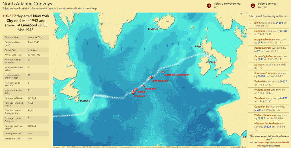
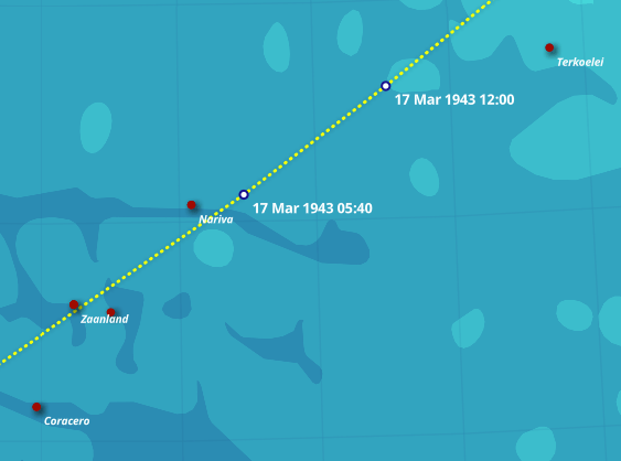
Convoy HX-229 departed New York City on 8 March 1943 with 40 merchant vessels and arrived in the UK 15 days later with only 26. One ship returned to New York City early on in the voyage and the other 13 were lost along the way, sunk by German U-boats. Along with the slower SC-122 convoy that left New York City 3 days earlier and lost 9 of its 51 ships, HX-229’s passage across the North Atlantic marked a low point in Allied fortunes in the North Atlantic battleground. Books (1, 2) have been written on the battles surrounding these two convoys and maps of their routes are easy to find online, including ones that are incorrect. Location and timing is crucial for the success of participants in any battle and providing maps showing these locations and their times is helpful in understanding how the battles of convoys HX-229 and SC-122 unfolded.

An Allied convoy near Iceland, 1942

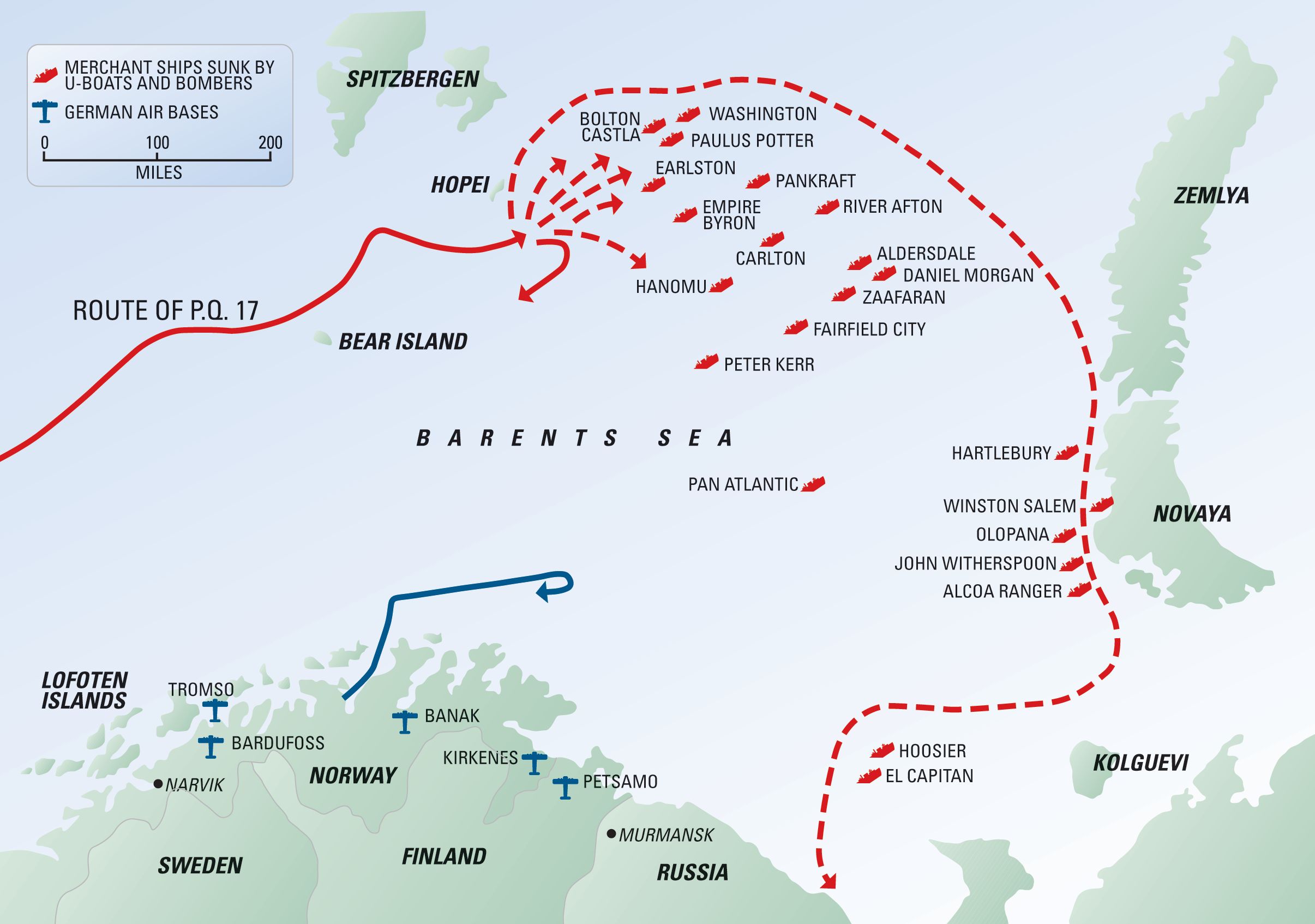
Other convoys that lost multiple ships have also been mapped and described. Convoy PQ-17, for instance, sailed for the Russian port of Arkhangelesk from Iceland in June/July 1942, lost 23 of its 35 merchant vessels to German U-boats and aircraft, and has also been written about (1, 2) and mapped (1, 2). But the majority of convoys have passed into obscurity.

This is not surprising as there were over 18,000 Allied convoys during the Second World War. Most of these convoys sailed undisturbed and arrived at their destinations unscathed. Of the 364 convoys that sailed as part of the HX series of convoys between September 1939 and May 1945, for instance, 299 did not lose any ship to Axis forces. In fact, close to 96% of the ships that sailed in these convoys arrived at their destination. Most of the ships that did not make the trip returned to the port of their origin due to mechanical or other issues. Less than 1% – 179 – of the 18,566 ships that sailed as part of an HX convoy were sunk due to enemy action. (Numbers have been compiled from Convoyweb).

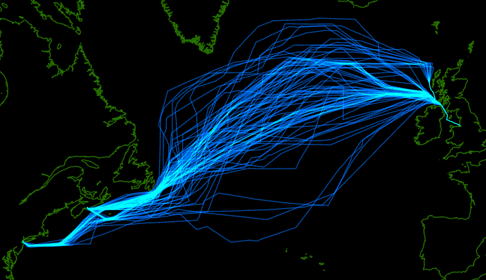
Maps for most convoys are difficult to find. This is understandable since most convoys arrived safely at their destinations without incident. But, though the maps of single convoys that had no losses might be somewhat mundane and dull to look at, collectively the alignment of their routes may tell a story.

The paths of 87 HX convoys HX 153 – HX 190, HX 192 – HX 219, HX 221 – HX 239, HX 245

About the World War II Convoy Atlas

The World War II Convoy Atlas is a collection of convoy maps in an interactive dashboard. Included in the Atlas so far are the routes of 100 convoys. Aside from the maps, the dashboard includes summary information on each convoy and a listing of any ships that were sunk along its route. Though there were 18,461 Allied convoys that sailed during World War II I don’t expect to be mapping them all. But do expect to see the number of convoys mapped increase over the next few months.

Included on the map are the following convoy routes:

  • HX 153 – 190, 192 – 239, 245
  • MW 12
  • ON 23, 127, 154, 166, 202
  • ONS 5, 18, 24
  • PQ 13
  • SC 103, 107, 121, 122

Explore the World War II Convoy Atlas.


The Data Sources

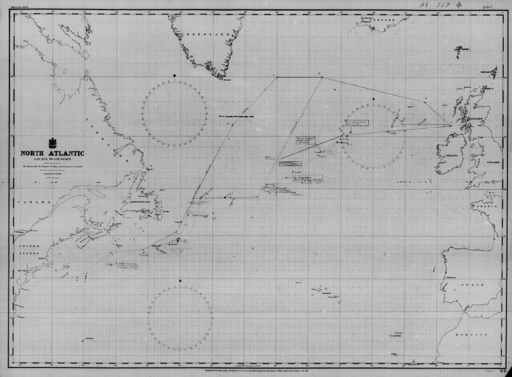
Much of the mapping information that is included in the Atlas comes from a single source I have recently discovered: the Royal Canadian Navy: Convoy Reports of Proceedings, 1939-1945. This collection includes messages between Canadian naval headquarters and the convoy commanders, convoy reports and maps on which both the planned and actual route of the convoy were plotted. This collection of wartime documents was captured on microfilm, after which the originals were destroyed. Library and Archives Canada has since digitized and published the microfilm.

The route map of Convoy HX-229. This sheet is the typical North Atlantic sheet used to record the trans-Atlantic convoys, probably has a scale of 1:8,000,000 (the numbers are difficult to read) and probably is about 107 cm (42 in) wide by 84 cm (33 in) high.
Source: Library & Archives Canada

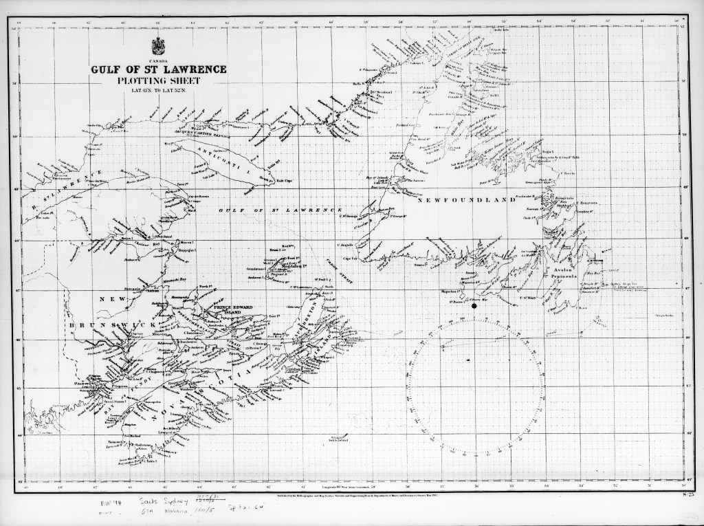
The collection contains over 223,000 images in 42 reels. There is no index to the images and the images are not searchable so finding specific content in the collection can be a challenge. The convoy maps, conveniently, appear in last 5 reels of the collection (C-5542 to C-5546). A complete list of the convoys mapped is provided the in table at the end of this post. The maps were published by the Hydrographic and Map Service in the Canadian government’s Department of Mines and Resources and were used by both merchant and naval vessels. The most common maps in the collection is one depicting the North Atlantic (example in the figure above) and one that depicts Atlantic Canada (see figure below). Captains and crewmembers would plot the expected route and the actual route, with dates and times. Sometimes additional notes were recorded to indicate events.

The route map of Convoy BW-94. This is the standard Gulf of St. Lawrence map that was used to plot the route of coastal convoys in and around Atlantic Canada and Newfoundland. The scale and size of this map is unknown. Source: Library and Archives Canada.

Putting the Atlas Together

Creating the convoy data required the published maps in the Collection to be imported and geo-referenced before they could be digitized. Summary information compiled from data published on ConvoyWeb was added to the appropriate record. The Sunken Ships database was added to a map. Since it shares a common data field with the convoy data, both could easily be incorporated into an interactive dashboard. This could easily have been done in one dashboard – an initially was.

But I split up the Atlas into 3 pages and, much like a paper atlas, each page focuses on one area or theatre of operations. Each map has its own map projection – one that is more suitable to the area of interest than the usual Web Mercator. This was especially true for the Arctic convoy map where east – west distances are grossly distorted in Web Mercator. Because the content of my map was fairly simple to begin with and because I didn’t need the wealth of information that comes with a standard basemap, I could dispense with the usual Web Mercator projection.

Instead I cached one single layer – my bathymetry data (from Natural Earth) that happened to draw faster in cached format anyway – in the projection I selected for the map. Because I had three different maps, each with a different projection, I had to do this 3 times. The caching time is quick and the storage required to host the cache is minimal so this was not onerous.

The maps for each theatre were placed in their own dashboards and each dashboard was given its own page within an ArcGIS Online Experience Builder app. As an introduction, a StoryMap was created and placed on the first page. Because of the flexibility of the Experience Builder app, it can be easily expanded to include additional content and enables a stable url regardless of the content changes within it.

Not a good day for HX-229

Index to the Library & Archives Canada convoy map collection
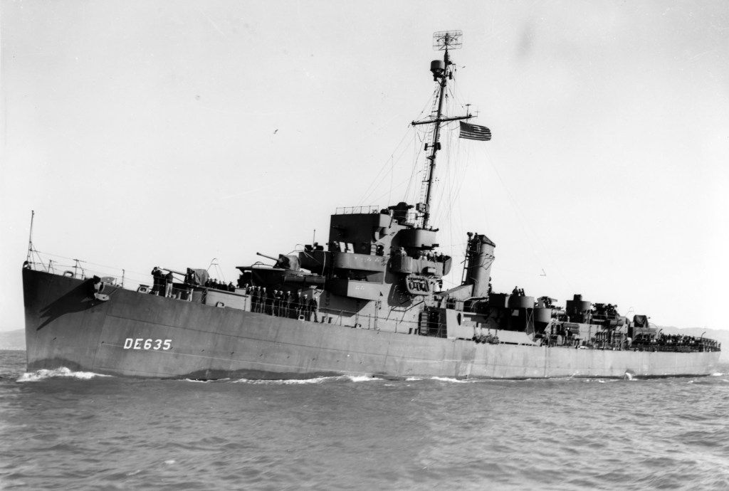
The following is a catalogue of the convoy maps that appear in the Library & Archives Canada collection published on Canadiana Héritage. Not all convoy sequences are complete.

Convoy Series Reel Images
AT-54A – AT-212 C-5542 1 – 275
BA-13 – BA-18 C-5542 276 – 281
BS-9 – BS – 102 C-5542 282 – 364
BW-30 – BW-181 C-5542 365 – 582
BX-57 – BX-164 C-5542 383 – 763
CK-1 – CK-3 C-5542 764 – 769
CU-3 – CU-73 C-5542 770 – 896
FH-60 – FH-122 C-5542 897 – 1044
FH-122A – FH-179A C-5543 1 – 80
GS-24 – GS-68 C-5543 81 – 160
GUF-10 – GUF-22 C-5543 161 – 187
GUS-8 – GUS-92 C-5543 188 – 339
HF-59 – HF-111 C-5543 340 – 497
HHX-220 C-5543 498 – 500
HJ-29 – HJ-101 C-5543 501 – 582
HJF-1 – HJF-48 C-5543 583 – 663
HL – 1 C-5543 664 – 665
HS-91A – HS-227 C-5543 666 – 869
HX-154 – HX-238 C-5543 870 – 1050
HX-239 – HX-359 C-5544 1 – 182
HXF-290 – HXF-310 C-5544 183 – 203
HXM-287 – HXM-304 C-5544 204 – 215
HXS-288 – HXS-303 C-5544 216 -228
IUS-3 – IUS-5 C-5544 229 – 235
JH-56 – JH-121 C-5544 236 – 357
JHF-1 – JHF-59 C-5544 358 – 452
JN-34 – JN-38 C-5544 453 – 463
LN-1 – LN-30 C-5544 464 – 497
NA-1 – NA-13 C-5544 498 – 517
NL-14 – NL-31 C-5544 518 – 556
NY-10 – NY-170 C-5544 557 – 589
ON-23 – ON-287 C-5544 590 – 1120
ON-287 – ON-305 C-5545 1 – 45
ONF-232 – ON-255 C-5545 46 – 70
ONM-153 – ONM-249 C-5545 71 – 87
ONS-1 – ONS-254 C-5545 88 – 222
OT-6 – OT-12 C-5545 223 – 239
QS-54 – QS-109 C-5545 240 – 305
SB-46 – SB-97 C-5545 306-372
SC-47 – SC-177 C-5545 373 – 639
SG-26 – SG-45 C-5545 640 – 677
SH-86A – SH-223A C-5545 678 – 930
SQ-36 – SQ-106 C-5545 931-998
SC-104 – SC-109 C-5545 999 – 1010
TA-50A – TA97A C-5545 1011 – 1083
TA-99A – TA-208A C-5546 1 – 200
TCU-23 – TCU-35 C-5546 201 – 214
TA-208B – TA-215 C-5546 215 – 217
TU-5 – TU-11 C-5546 218 – 257
UC-3 – UC-70B C-5546 258-415
UCT-23 – UCT-35 C-5546 416 – 429
UGF-9 – UGF-22 C-5546 430 – 460
UGS-10 – UGS-95 C-5546 461 – 604
UT-1 – UT-14 C-5546 605 – 624
WB-23 – WB-171 C-5546 625 – 829
XB-58 – XB-165 C-5546 830 – 1011
YD-2 – YD-4 C-5546 1012 – 1017
     

April 2024 Updates

The following changes have been made to the database:

  • 8 records edited (additional links, corrections)
  • 3 records moved to better locations
  • 5 records added

The following sunken vessels were added to the map:

  • Dalny, sunk 4 June 1943
  • Gonneville, sunk 20 August 1944
  • H23 Grandlieu, sunk 20 June 1944
  • Molch, sunk 2 May 1945
  • Taurus, sunk 7 July 1944

See them on the map.

Mapping U-boat KTB Locations

Abstract

This article examines the challenges and accuracy of recording U-boat positions during World War II, using U-156’s fourth war patrol as a case study. It explores the navigation methods employed, including celestial navigation, dead reckoning, and radio direction-finding, shedding light on the limitations and accuracy of each. The German naval grid system is discussed, highlighting its role in securing positions but also its potential for introducing errors. The study analyzes errors in position recording, emphasizing the impact of atmospheric conditions, recording errors, and map reading difficulties. The conclusion underscores the complexity of obtaining precise positions during wartime and questions the effectiveness of the German naval grid system in achieving its intended purpose.

Time to read: 24 minutes


Introduction

On June 3rd, 1943, the Greek merchant ship Boris was sailing alone and unescorted in the South Atlantic Ocean. It had set out from Santos, Brazil with a cargo of bauxite, wood and castor seed a few days before and was making its way to Freetown, Liberia where it was to join a convoy for Northern Ireland. At 23:40[1] the Boris was hit by one of three torpedoes fired by the German submarine U-180. The ship began to sink and the crew of 37 safely evacuated to two lifeboats before the submarine finished off the ship with two more torpedoes. The Germans questioned some of the crew and the U-boat departed, leaving the two lifeboats to make their own way to safety.

Figure 1: Boris, a 5,166-ton Greek cargo vessel. Photo: uboat.net

The two lifeboats parted ways; one was picked up by the British ship Cambria 11 days later 15 miles from Recife, Brazil, and the rescued crew were put ashore there. The other was rescued by the Spanish passenger ship Cabo de Bueno Esperanza on June 17 and landed in Rio de Janeiro. There were no casualties.

Although the crew of the Boris knew that their ship was sunk somewhere west of Ascension Island, the exact location remained unknown until after the war when it was possible to access the war diary of U-180. The U-boat placed the sinking at 7° 14’S, 18° 41’W, about 250 nautical miles (nmi) west of Ascension and about 1000 nmi east of Recife, Brazil.

Figure 2: Location of the sinking of Boris, based on U-180’s KTB

Apart from the survival of the Boris’ crew, this is not an unusual story from the Second World War. German U-boats sank 2,937 ships during the course of the war, and about two-thirds of these (estimates are vague) were sailing independently and unescorted. Ships under attack often sent out distress signals by radio with their latest known position, something that may have already been a few hours old. Because of the limited range of merchant vessels’ radio transmitters, these distress messages would sometimes be picked up by other vessels or radio receivers on the area. Many times they were not. And, in these cases, the only record of the location of a ship’s sinking was in the war diaries (Kriegstagebücher or KTB) of the attacking German U-boats.

How accurate were these KTBs, and how reliable are they as sources of wartime data? To get a better understanding, we must consider how the positional data recorded were arrived at, who did the recording and for what purpose.


Navigation Technology in World War II

Taking One’s Position

In the current era of cellphones and GPS, it is easy for anyone to determine their geographic position within five metres. During the Second World War,, navigation employed several different technologies, some of which had been in use for hundreds of years, and none of which provided an accuracy comparable to what we have access to today.

Figure 3: An example of a German sextant used by U-boats during World War II. Photo: KM-Spain / Gentleman’s Military Interest Club

The primary method of calculating marine position during the Second World War was celestial navigation. Using a sextant (Figure 3) and an accurate timepiece, sailors calculated their position anywhere on the globe — provided the sky was at least partially clear. With a fix on a celestial object, navigators consulted sight reduction tables and calculated longitude and latitude values that, under ideal conditions, provided positional accuracy within 5 nmi. [2] Wartime, particularly during stormy winter months on the North Atlantic, seldom provided ideal conditions, however, and surface vessels fared no better than U-boats in obtaining an accurate position.[3]

Because vessels at sea were always moving, it was impossible to take multiple readings to verify a position. Instead, two sailors would take a reading simultaneously and average their calculations to arrive at a position.

In unfavourable atmospheric conditions, when celestial navigation wasn’t possible, sailors calculated their position using a technique called dead reckoning. Sailors took the vessel’s last recorded position and calculated the distance travelled since (speed x time), factoring in direction and the estimated speeds of ocean currents and wind to arrive at an estimated position. Closer to shore, sailors confirmed the position they arrived at by dead reckoning by comparing it to what appeared on a nautical chart for the area and identifying one or two sighted landmarks. Dead reckoning was only as accurate as the previous navigation fix; the greater the timespan between, the less the accuracy. A battle, with its rapid directional changes and confusion, complicated calculations.[4] Still, an estimated positional reading was better than none.

Celestial readings could be taken while a U-boat was underwater through the use of the submarine’s observation periscope, but these periscopes became unusable at speeds of 6 knots or more because of vibrations and were prone to fogging up, limiting their use.

Another tool that was available was radio direction-finding. By receiving radio signals from two different known locations, a vessel could triangulate its position. Conversely, a radio signal from any unknown point of origin could be pinpointed if it was received at two known locations. The latter was frequently used by the Allies during the war to locate U-boats as the latter regularly communicated by radio with their home base.

KTBs rarely indicate which position-fixing method was used. A few KTBs do note celestial navigation fixes or shore readings. Kriegsmarine protocol required that positions be recorded every four hours and for significant events but did not specify how these positions were to be calculated. One U-Boat officer writes, “For days we had no proper navigational fix. We could not shoot a single star, nor did we see the sun or the moon.”[5] In this case, all the positions were calculated by dead reckoning. As the war progressed and Allied escort vessels and aircraft were increasingly successful in forcing U-boats to submerge more frequently and for longer periods, celestial navigation became less frequent.

Recording a Position

A positional reading was normally recorded in latitude and longitude values (degrees and minutes; seconds were rarely seen in maritime and naval logs of the time), allowing a granularity of up to 1 nmi between positions. In reality, this level of granularity was rarely achieved by U-boats because of the already mentioned limitations in the available technology.

Latitude and longitude coordinates were used by the Germans but, more often, positions recorded by vessels of the Kriegsmarine, including U-boats, used the German navy’s naval grid system. The marinequadratkarte system, initially developed by the Luftwaffe prior to the war and adopted by the Kriegsmarine, split the world into quadrants that were identified using a two-letter code (Figure 4). Each of these quadrants was split into 81 equal-sized squares, identified by a two-digit number (zeroes were not used; Figure 5). These were split again, into 81 even smaller squares, also identified by two-digit numbers (Figure 6). These squares were 6 nmi in height and width, varying somewhat according to how far a given square was from the equator. By this method, the Kriegsmarine could identify any location in the world within 6 nmi using a combination of 6 letters and digits.

Figure 4: The Kriegsmarine’s naval grid system for the world, showing all the 2-letter named quadrants.
Figure 5: A section of a Kriegsmarine chart of the North Atlantic, showing the two-letter named quadrants and their 2-digit sub-squares. This map was produced at a scale of 1:17,500,000 (Nr. 3401 Klein Nord-Atlantischer Ozean, 1941)
Figure 6: A sample of the chart for the Caribbean Sea, Gulf of Mexico and western central Atlantic Ocean. This is displayed at scale (1:3,300,000; image displayed is 12.7 cm x 12.7 cm) and each of the smallest grid squares is about 3.5 mm in width. Havana, Cuba, highlighted in red in the lower part of the map, is at square DM4389 (George A Smathers Libraries, University of Florida, Nordatlantik Amerikanisches Mittelmeer, 1943)

This alphanumeric string was adopted as an additional security measure to make it more difficult for the Allies to locate a vessel should the message be intercepted and decoded. However, parts of the Marine Quadratkarte fell into British hands before the end of 1939 system and by the following summer the Allies had enough information to decode positions described by the Marine Quadratkarte system across the North Atlantic and the Mediterranean.[6] in an attempt to further confuse their enemies, the Germans later scrambled the grid square values that were radioed to home base but the actual, correct grid square value of the U-boat’s position was always recorded in the KTB.[7]

The crew tasked with recording the U-boat’s position in the KTB had two steps to complete: position the U-boat correctly on the map and calculate the corresponding Kriegsmarine grid square correctly. These were then written into the KTB, next to the time and notes on the voyage. Often, the grid square was shortened to the last four digits, with the assumption that the boat was still in the same quadrant as the previous entry (see Figure 7 & 8).

Figure 7: A sample of U-156’s KTB for its 4th patrol. This shows the times, recorded locations and events of October 2, 1942. Note how the Kriegsmarine grid square reference has been shortened to a 4-digit number in the second column. Note also the comments in the third column where latitude and longitude coordinates are provided.
Figure 8: Uboatarchive.net’s English translation of the same page shown in Figure 2. Note how the editors have re-added the 2-letter quadrant name before the 4-digits.

The KTB

The U-boat commander wrote the KTB, drawing on the diaries of the other officers on the boat. It was usually written during the voyage shortly after the events had transpired. The navigator passed positional information to the commander for entry into the handwritten patrol log; this log was typed up by a crew member once the vessel returned to port. Herbert A. Werner, serving as a watch officer on U-557 under Ottokar Paulssen, writes how he “typed the final version of the Captain’s logbook and the Chief’s reports, wrote a full accounting of the disposition of each torpedo, and made detailed diagrams of U-557‘s entire route and each of the attack patterns Paulssen had used.”[8] Once completed, the captain reviewed and signed the KTB before passing it on to the Kriegsmarine operations staff for their review, analysis and archiving. It was not uncommon for Admiral Karl Dönitz, commander of the Kriegsmarine’s U-boat arm and, later, Commander-in-Chief of the navy, to review the KTB of a just-completed patrol with the U-boat’s commander.[9] Because the log was not so much an ongoing account as events unfolded but more of an after-the-fact retelling, errors could be corrected before they were recorded in the KTB. Even so, errors did occur.


Case Study: U-156’s Fourth War Patrol KTB

Background

Of the thousands of U-Boat KTBs available to consider, I chose U-156’s fourth war patrol because it contains both latitude and longitude coordinates and the grid square values in many of the same entries as well as indicating how those positions were arrived at. Some KTBs include both latitude and longitude coordinates and grid squares, but few indicate how those positions were arrived at. This is important as position fixing via celestial readings is more accurate than dead-reckoning, allowing us to better judge the accuracy of the recorded positions. Including both latitude and longitude coordinates and grid square values for the same position also allows for comparison of the two.

U-156 departed Lorient, France on 20 August 1942 and returned to it 87 days later on 16 November 1942. Commanded by 34-year-old Werner Hartenstein, it sank three vessels during this, its fourth war patrol, but the voyage is probably best remembered for the sinking of the British passenger ship Laconia, which carried more than 2,700 crew and passengers, of whom 1,800 were Italian prisoners of war. U-156 spent some days looking after survivors of the Laconia until Vichy French vessels could rescue them. Though the U-boat was clearly marked with a Red Cross and was surrounded by Laconia survivors on rafts and on the deck of the submarine, it was attacked by an American aircraft. The incident spurred the Kriegsmarine to order its submariners not to provide any kind of aid to the survivors of ships that they sank.

Figure 9: A photo taken from the conning tower of U-156, showing U-507 and many of the survivors of the Laconia, sunk earlier by U-156.
Table 1: A Summary of the positions of U-156’s 4th war patrol as recorded in the KTB

U-156’s KTB for this particular patrol includes 729 position entries, 106 of which include both a grid square coordinate and a latitude and longitude coordinate. Most of the latitude and longitude coordinates are stated as navigation fixes – that is, they are based on readings of celestial objects. On this patrol, the navigation fixes were generally taken early to mid-morning and late in the evening.

Plotting the Data from the KTBs

The source data for this KTB are scanned copies of the original German versions. In some cases the scans were not well done, resulting in text being partly cut off or, in some cases, illegible.

Using an online application like Naval Grid Calculator, it is easy for us today to derive latitude and longitude values from the Kriegsmarine grid coordinates stated in the U-boat log without having to refer to any maps. The resulting coordinates, along with those provided in the KTB as part of the regular navigational fixes, were plotted on the map.

Errors in the KTB

U-156’s KTB has errors in some of the positions that are recorded. An initial plot of both the latitude and longitude coordinates and the grid square coordinates makes some of these errors immediately obvious. The map below (Figure 9) highlights some of those issues and the corrections that were made. The KTB contained 9 such errors, or 1.1% of the location references recorded in the log.

Figure 10: U-156’s positions as they are recorded in its KTB.
Arrows indicate where erroneous positions were corrected to.

The 6 points clearly out of position in U-156’s plot (Figure 10) off the coast of northwest Africa illustrate a common type of error. These 6 positions occur in chronological sequence, beginning with 31 October 1942 16:00 and running to 1 November 1942 09:18. In the KTB the position recorded for midnight on October 31st is recorded using 6 digits to identify the Kriegsmarine grid square (EJ 7685; see Figure 11). The next recorded position, taken 4 hours later, only uses the last 4 digits of the Kriegsmarine grid square, the assumption being that it falls within the same 2-letter quadrant (in this case, EJ). This shortening of the grid square coordinates occurs in most U-boat KTBs, including that of U-156. At 16:00, the grid square is again recorded using 6-digits but this time the crewmember recording the position mistakenly indicated that the Kriegsmarine quadrant was DJ. As a result, all subsequent positions in the KTB are assumed to be within this quadrant until a new quadrant is recorded. This does not occur in the log until noon on November 1st when the position is recorded as EH6634. From this point on, the positions are assumed to be in the EH quadrant.

Figure 11: Extract from page 39 of U-156’s KTB for its 4th war patrol. Note also the poor quality of the scan

Moving these 6 positions over from quadrant DJ to EJ, the same quadrant as the preceding positions, makes sense, as shown in Figure 13.

Figure 13: Moving the 6 suspect positions off the coast of northwest Africa in quadrant DJ (top right) to quadrant EJ (bottom left) fills the gap in U-156’s route map and aligns with the positions recorded both before and after (numbers refer to the chronological order in which they appear in the KTB).

The errors are not restricted to the 6-digit grid square references but also occur with the recordings of the latitude and longitude coordinates. Two such cases appear in U-156’s KTB. In both cases, a single digit of the two coordinate pairs was different than what it should have been, resulting in both locations being offset by 1º of latitude.

Comparing Latitude & Longitude Coordinates and Grid Squares

There are 106 entries in the KTB that include both latitude and longitude coordinates and grid square references, providing the opportunity to determine how closely they align with each other. In an ideal world, each latitude and longitude coordinate would fall within its corresponding grid square. But this is not the case.

Table 2 highlights how closely the latitude and longitude coordinates match with the grid square referenced in the same KTB entry. Both the latitude and longitude coordinates and the grid square coordinates are the corrected ones; that is, those errors mentioned earlier were fixed for this comparison. There were 59 cases where the latitude and longitude coordinates fall within the grid square mentioned in the same entry – a match rate of 55%. If we consider that a navigation fix can be within 5 nmi of the actual location, then the possibility that the fixed position falls within the grid square rises to 95%.

Table 2: Matching Rates of Lat-Long & Grid Square Coordinates
Figure 14: A sample of the comparison between the longitude and latitude coordinates and the grid squares for U-156.

Other Vessels

U-156 encountered 9 different vessels during its 4th war patrol – 6 other U-boats and 3 Allied merchant vessels which it torpedoed and sank. Each of those 6 U-boats also recorded times and positions in their KTBs using grid square coordinates. U-156 met U-68 on 3 different occasions and U-506 twice. All of the other U-boats it met once during its patrol. In a perfect world the positions recorded in U-156’s KTB should match up to the positions of the U-boats it met up with. However, this is not the case.

Table 3: Distance between Recorded Positions of Meeting Points

Each encounter that U-156 had with another U-boat on its 4th war patrol is listed in Table 3. The position of each grid square is assumed to be the centre of the grid square. The only location that was not arrived in this manner are the second set of coordinates provided by U-506 that supplied both latitude and longitude and grid square coordinates in the same entry. The rest of the positions could be anywhere with the 6 nmi x 6 nmi square that is referred to, meaning that any two points could be up to 17 nmi apart, if you consider that the points could be in opposite ends of their grid squares. All but two of the location pairs in the table fall within this margin of error. U-125’s position has been corrected to FE 1223 from ET1223, the grid square recorded in its log. The recorded – and uncorrected – position would place the boats 8 degrees or 463 nmi apart!

It should be noted that an observer on a U-Boat conning tower is about 5 metres above the surface of the water. At that height the farthest a sharp-eyed crewmember could see is about 13.3 nmi, something that would only happen when atmospheric conditions were perfect. This would suggest that the positions of the 2 boats would need to be no more than 13.3 nmi apart to be considered to be in the same place. In the cases of the 2 U-boats that recorded their positions more than 13.3 nmi apart (positions 1, 2 and 7 in Table 3), one or both logged an incorrect location in their KTB. For two other pairs of positions (positions 5 & 8) that are around 12 nmi apart, this is probably the case as well. That would mean that of the 18 positions recorded here, 5 to 10 of the positions recorded were incorrect – not a statistic that would suggest a high level of accuracy.

One other comparison for U-156 can be made. During the sinking of the Laconia, the passenger ship sent out a distress call with its location. At 22:07 on the 19th of September, U-156 recorded its position as FF7721 (4.85S, 11.45W). At 22:22, the Laconia sent out a distress call stating its position to be 4.56S, 11.42W, a distance of 17 nmi from U-156’s stated position 15 minutes earlier.


Discussion

Morgan & Taylor write that “the sinking coordinates for any warship lost on the high seas should be regarded as conjectural at best,”[10] whether those coordinates came from the U-boat’s themselves or from the enemies they faced. A review of U-156’s KTB for its 4th war patrol seems to support that assertion.

Errors appearing in U-156’s KTB can be split into 3 different categories: the accuracy of the processes used to arrive at a stated position, recording errors and map reading errors.

Accuracy of Position Calculations

As mentioned earlier, positions recorded in the KTB were arrived at using 3 different methods: celestial navigation, dead reckoning and shore readings. As stated earlier, using a sextant generally provides results with 5 nmi but this can vary considerably, depending on the atmospheric conditions. Dead reckoning, usually based on navigation fixes from a preceding time, are no more accurate than these navigation fixes and are generally worse, depending on the length of time that separates them from their predecessors. The two positions listed in U-156’s KTB based on shore readings are not recorded in latitude and longitude values but only as a bearing and distance to a sighted landmark so there is no way of determining their accuracy.

Recording Errors

Figure 15: The track chart of U-156’s 4th war patrol with relevant two-letter quadrants. A track chart was one of the Kriegsmarine’s requirements of a U-boat patrol and often accompanied the KTB itself. Note that there do not appear to be any misplaced positions on the map that were noted earlier.

As noted earlier, just over 1% of the positions recorded in U-156’s KTB are what can be called recording errors – a rate that could be considered acceptable.[11] It is possible that the crewmember recording the position in the log unintentionally recorded a wrong number or letter in the log. In the case of the 6 positions off the coast of northwest Africa, this was probably an oversight. These incorrect positions do not appear to have affected the creation of the route map that is attached to the KTB (see Figure 15).

Map Reading Errors

Herbert Werner writes about his experience aboard U-230 in February 1943 that was probably typical of the experience of many U-boat crews: “As we pushed through the heavy seas toward our assigned position 600 miles east of Newfoundland, conditions worsened rapidly aboard U-230. Water that poured in through the open hatch sloshed around our feet, and the high humidity within the hull caused food to rot, the skin to turn flabby, and our charts to dissolve.”[12] Heat and humidity would likely have been worse in the tropics where U-156 was operating for most of its 4th war patrol, making conditions for detailed map reading even more difficult.

The process of arriving at a grid square coordinate for the boat’s location, in the case of a navigation fix, required the crewmember to determine the location of the latitude and longitude coordinates on the map, then to interpret which grid square applied. Naval grid charts were provided to the U-boats of more distant waters like the South Atlantic at a scale of 1:3,300,000. Grid squares at that scale would be 3.5 mm in width on the map, leaving plenty of room for error in determining the correct grid square. If the number of latitude and longitude coordinates in U-156’s KTB that do not fall within their corresponding grid square is any indication (44.3%), errors because of inattentive map reading, or incorrect map interpretation, occurred frequently.


Conclusion

The insights gained from a look at one U-boat KTB, cannot necessarily be extrapolated to the rest of the U-boat fleet throughout the war. The quality of the data in a KTB depended on the knowledge and experience of those recording the information contained therein. As the war progressed, more and more experienced U-boat crews suffered a deadly end and conditions for the remaining, less experienced crews became less favourable to accurate position taking. A comparison of U-156’s KTB, written by a commander and crew with experience on 3 war patrols in fairly favourable conditions to that of another, first time commander and crew later in the war that was constantly under threat of attack, may shed light on both the effect of inexperience and wartime conditions on the recording of U-boat positions.

There will be errors in any ship’s log, particularly during wartime or adverse weather conditions. The accuracy of any ship’s recorded position during the Second World War is not likely to be better than +/- 5 nmi unless radio direction was being used. The German Naval Grid System, however, did not improve matters at all for the U-boats at sea. Meant to cloak a U-boat’s position from its enemies, the Naval Grid System was an unnecessary complication that failed to disguise U-boat’s positions and, instead, clouded their accuracy.


Footnotes

[1] All times are Central European Time, GMT – 1, unless otherwise stated.

[2] The Institute of Navigation. Weems, Averaging Bubble Sextant Observations. See also the discussion at CruisersForum.

[3] Morgan, Daniel & Taylor, Bruce, U-boat Attack Logs: A Complete Record of Warship Sinkings from Original Sources 1939 – 1945, p. xviii

[4] Uboat.net

[5] Werner, Commander Herbert A., Iron Coffins, p. 27

[6] Morgan & Taylor, p. xviii

[7] Morgan & Taylor, p. xxxv

[8] Werner, p. 49

[9] Gannon, Michael. Operation Drumbeat, p. 52.

[10] Morgan & Taylor, p. xviii

[11] Uboatarchive.net’s English translation of U-156’s KTB contains 5 grid square positions that are different from what appears in the scanned German version of the KTB – an error rate of 0.7% for a process that occurred in far more amenable conditions than on a U-boat at sea. My own process of transcribing the positions resulted in a few errors that I was able to fix, having had the luxury of time to do so.

[12] Werner, Iron Coffins, pp. 89-90.

February 2024 Updates

The following changes have been made to the database of sunken ships:

  • 6 records edited (additional links, corrections)
  • 4 records moved to better locations
  • 1 record deleted
  • 7 records added

The following sunken vessels were added to the database:

  • Bahia Castillo, sunk on 1 May 1940
  • Berlin, sunk on 1 February 1945
  • Nioi, sunk on 29 October 1943
  • RD-4, sunk on 29 January 1943
  • Sifnos, sunk on 4 March 1944
  • U-1407, sunk on 4 May 1945
  • U-4708, sunk on 9 April 1945

See them all on the map.

January 2024 Updates

A shorter list of updates to the database for January.

  • 5 records edited (additional links, corrections)
  • 1 record moved to a better location
  • 1 record deleted
  • 10 records added

The following sunken vessels were added to the database:

  • Kentucky, sunk 15 June 1942
  • TA 24 Arturo, sunk 18 March 1945
  • TA 29 Eridano, sunk 18 March 1945
  • U-684, sunk 3 May 1945
  • U-685, sunk 3 May 1945
  • U-2501, sunk 3 May 1945
  • U-2505, sunk 3 May 1945
  • U-3504, sunk 3 May 1945
  • U-3506, sunk 3 May 1945
  • Volante, sunk 12 July 1940

Read about the discovery of the 6 U-boats mentioned here that were scuttled at the end of the war in Europe in the U-boat bunkers in Hamburg.

December 2023 Updates

Updates for this month:

  • 19 records edited (additional links, corrections)
  • 2 records moved to better locations
  • 1 record deleted
  • 20 records added

The following sunken vessels were added to the database:

  • Ausonia, sunk 18 September 1944 (Read about it on Instagram)
  • Eso, sunk 19 January 1943
  • Giansone I, sunk 24 October 1940
  • La Galissonnière, sunk 18 August 1944
  • Macallè, sunk 15 June 1940
  • Riccardo Grazioli Lante, sunk 24 August 1941
  • Strasbourg, sunk 18 August 1944 (Read about it on Instagram)
  • Stromboli, sunk 19 January 1943
  • Volta, sunk 8 October 1943
  • MAS 537, sunk 4 September 1940
  • MAS 552, sunk 30 April 1943
  • MS 25, sunk 30 April 1943
  • MS 33, sunk 3 November 1943
  • MZ 723, sunk 4 August 1942
  • MZ 733, sunk 21 May 1943
  • MZ 771, sunk 7 April 1943
  • RD 22, sunk 25 October 1943
  • RD 7, sunk 15 June 1942
  • VAS 225, sunk 5 May 1943